
Problem: Design a petabyte-scale data warehouse for analytics.
Key Considerations:
- Columnar storage (Parquet/ORC) for analytical query efficiency
- ETL/ELT pipelines using Apache Airflow for orchestration
- Star schema or Snowflake schema for dimensional modeling
- Partitioning and clustering strategies for query performance
- NFRs: Query performance, storage cost optimization, data freshness SLAs
High Level Architecture
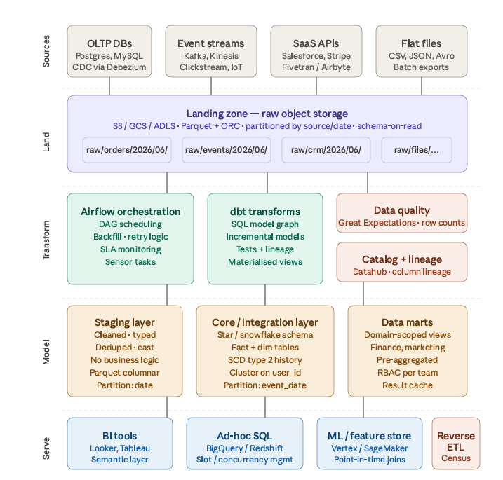
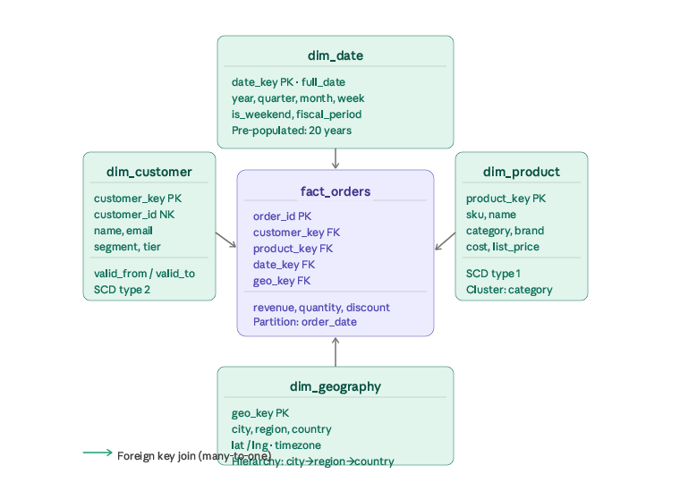
The star schema is the structural heart of the core layer. Here’s how fact and dimension tables relate:
Design breakdown
Columnar storage — Parquet / ORC
At petabyte scale, the storage format is a first-order performance decision. Columnar formats let the query engine skip entire column chunks it doesn’t need. A query like SELECT SUM(revenue) WHERE region = 'EU' reads only two columns regardless of how many others exist. Key choices:
- Use Parquet with Snappy compression as the default — broad ecosystem support, excellent read performance, and ~30–40% space saving over raw CSV.
- Use ORC for Hive-heavy stacks; it has slightly better predicate pushdown in some engines.
- Target row group sizes of 128–512 MB — too small and metadata overhead dominates; too large and partial reads become expensive.
- Enable column statistics (min/max per row group) so query engines can prune without reading data.
Partitioning and clustering
These two techniques eliminate data scanned at different granularities:
Partitioning splits the physical file layout by a column value. event_date is the universal partition key — nearly every analytical query has a date predicate. A query for last 7 days scans exactly 7 partitions regardless of how many years of history exist.
Clustering (BigQuery) or sort keys (Redshift/Snowflake) physically co-locate rows with similar values within a partition. Clustering fact_orders on (customer_id, product_category) means a query filtering on those columns reads a dense band of data rather than random rows across the partition. The rule of thumb: partition on the coarsest filter (date), cluster on the most selective filter in JOINs (foreign keys).
ELT orchestration with Airflow
Modern warehouses favour ELT over ETL — load raw first, transform inside the warehouse using its own compute. Airflow coordinates this:
- DAG design: one DAG per domain (orders, events, CRM), each with three task groups — ingest, validate (Great Expectations), transform (dbt run).
- Sensors:
S3KeySensororBigQueryTableSensorwaits for upstream data before proceeding, replacing fragile time-based scheduling. - Backfill: Airflow’s
catchup=True+start_datelets you replay any historical window when a business logic change requires reprocessing. - SLA miss callbacks: alert to PagerDuty if a critical table hasn’t refreshed by its SLA deadline.
Dimensional modeling — star vs snowflake
The star schema (shown above) is the right default. Each dimension joins to the fact table in a single hop. Query planners love it; analysts understand it; BI tools generate efficient SQL against it.
A snowflake schema normalises dimensions further — dim_product splits into dim_product + dim_category + dim_brand. This saves storage on low-cardinality repeating values but adds joins. At petabyte scale, storage is cheap; join latency is not. Start with star; snowflake only when a dimension table itself exceeds tens of millions of rows.
SCD Type 2 (Slowly Changing Dimensions) is the critical pattern for dim_customer. When a customer changes segment, insert a new row with a new surrogate key, update valid_to on the old row, and mark the new row is_current = true. Every historical fact row retains its foreign key to the customer’s state at the time of the event — analytically essential for cohort analysis.
NFR design choices
Query performance: result caching in data marts handles repeated dashboard queries; materialized views for expensive aggregations; BI semantic layer (Looker LookML, dbt metrics) centralizes business logic so every tool produces identical numbers.
Storage cost optimization: lifecycle policies move cold Parquet files to object storage cheaper tiers after 90 days. Pre-aggregated rollup tables (daily/weekly/monthly) mean 90% of BI queries never touch the raw fact table at all. Aggressive partition pruning and column pruning via the query engine’s predicate pushdown keep slot/byte costs controlled.
Data freshness SLAs: tiered by use case — streaming pipelines (Kafka → landing → staging) deliver operational metrics at sub-hourly latency; nightly Airflow DAGs refresh the full star schema by 6 AM; pre-aggregated mart tables refresh hourly using incremental dbt models that process only new rows since the last watermark.